
Comparing Free geocoding engines
Introduction
I have been struggling with geocoding for about a year now, and have begun to learn far more than I wanted about the ugly details of the tools available for free. In particular I have been using Google and the US Census Bureau for geocoding. They each have their own strengths and weaknesses, so I thought it would be appropriate to share what I have learned.
I would call Google promiscuous - they will try very hard to return a location to you, even if it is all wrong. So using Google, in my experience, requires a fair bit of post-processing. Of course, you are also limited to 2500 queries per 24 hours with Google, which can be a bummer.
The Census geocoder, on the other hand, is pretty restrictive. If the address isn’t pretty close, it will return nothing. This can be frustrating and require quite a bit of pre-processing, but it is nice that you can generally, with some caveats, trust the result.
So lets go through the two engines in more detail, with real examples.
library(gt)
library(tidyverse)
library(lubridate)
library(ggplot2)
library(magick)
library(tidyr)
library(scales)
library(ggmap)
library(sf)

caption = "Alan Jackson, Adelie Resources, LLC 2019"
theme_update(plot.caption = element_text(size = 7 ))

googlekey <- readRDS("~/Dropbox/CrimeStats/apikey.rds")

knitr::opts_chunk$set(echo = TRUE,
                      results='hide',
                      warning=FALSE,
                      message=FALSE)
Google Geocoding
Google requires you get an API key from them in order to do geocoding. This has been well-documented elsewhere, so I will not do that here.
What Locations do Google and the Census actually return?
Let’s generate a detailed map and see where the locations Google and the census gives us actually are. You might be surprised, even disturbed.
#   Some test addresses

Addresses <- c("303 Jackson Hill St, Houston, TX, 77007",
               "318 Jackson Hill St, Houston, TX, 77007",
               "320 Jackson Hill St, Houston, TX, 77007",
               "403 Jackson Hill St, Houston, TX, 77007",
               "404 Jackson Hill St, Houston, TX, 77007",
               "407 Jackson Hill St, Houston, TX, 77007",
               "413 Jackson Hill St, Houston, TX, 77007",
               "415 Jackson Hill St, Houston, TX, 77007")

# Set up the basemap

register_google(key = googlekey)
MapCenter <- c(-95.401650, 29.76480)
zoom <- 19
  gmap = get_map(location=MapCenter,
                 source="google",
                 zoom=zoom,
                 maptype="roadmap")
Here is my function for querying the census data
There is a good bit of error checking, retries, and tests
GetResult <- function(urlreq) {# query census server and retry
  #  required libraries

  require(httr)

  #   set up to retry twice on server type error (which usually works)
  attempt <- 1
  result <- tibble(status_code=0)
  while(result$status_code!=200 && attempt<=3 ) {
    if (attempt>1){print(paste("attempted", attempt))}
    attempt <- attempt + 1
    try(
      #     Go get result
      result <- httr::GET(urlreq)
    )
  }
  return(result)
}

Census_decoder <- function(address, city=NA, state=NA, zip=NA){


  urlreq <- paste0("https://geocoding.geo.census.gov/geocoder/geographies/address?street=",gsub(" ", "+",address))
  if (!is.na(city)){urlreq <- paste0(urlreq,"&city=", city)}
  if (!is.na(state)){urlreq <- paste0(urlreq,"&state=", state)}
  if (!is.na(zip)){urlreq <- paste0(urlreq,"&zip=", zip)}
  urlreq <- paste0(urlreq,"&benchmark=Public_AR_Current&vintage=Current_Current&format=json")

  print(urlreq)
  result <- GetResult(urlreq)

  #     did we succeed?
  if (result$status_code != 200) { # failure
    return(tibble(
      status=paste("fail_code",result$status_code),
      match_address=NA,
      lat=NA,
      long=NA,
      tract=NA,
      block=NA
    ))
  } else {
  result <- httr::content(result)
  Num_matches <- length(result[["result"]][["addressMatches"]])

  if (Num_matches <= 0) { # failed to find address
    return(tibble(
      status="fail_length no matches",
      match_address=NA,
      lat=NA,
      long=NA,
      tract=NA,
      block=NA
    ))
  }
    # pick matching result if multiples offered
  for (i in 1:Num_matches) {
    temp <- result[["result"]][["addressMatches"]][[i]]
    if (grepl(address,
        str_split(temp[["matchedAddress"]], ",")[1])) { break }
  }
    tract <- temp[["geographies"]][[
                   "2010 Census Blocks"]][[1]][["TRACT"]]
    if (is.null(tract)){
      return(tibble(
        status="fail_tract no tract",
        match_address=NA,
        lat=NA,
        long=NA,
        tract=NA,
        block=NA
      ))
    }
    status <- "success"
    match_address=temp[["matchedAddress"]]
    lat=temp[["coordinates"]][["y"]]
    lon=temp[["coordinates"]][["x"]]
    tract=temp[["geographies"]] [[
                "2010 Census Blocks"]][[1]][["TRACT"]]
    block=temp[["geographies"]] [[
                "2010 Census Blocks"]][[1]][["BLOCK"]]

    return(tibble(
      status=status,
      match_address=match_address,
      lat=lat,
      lon=lon,
      tract= tract,
      block=block
    ))
  } # end if/else
}
Here is code for decoding a google query
This assumes using the geocode call from ggmap
#   Function for pulling fields out of nested lists returned by geocode
getfields <- function(x){
              if(! is.na(x) && length(x$results)>0)  {tibble(
              lat=as.numeric(x$results[[1]]$geometry$location$lat),
              lon=as.numeric(x$results[[1]]$geometry$location$lng),
              types=x$results[[1]]$types[1],
              match_address=x$results[[1]]$formatted_address,
              LocType=x$results[[1]]$geometry$location_type)
              } else if ("status" %in% names(x) && x$status=="ZERO_RESULTS"){
                tibble(types=x$status,lat=NA,lon=NA, match_address=NA,LocType=NA)
              } else{
                tibble(types=NA,lat=NA,lon=NA, match_address=NA,LocType=NA)
              }
}
Let’s put points on a map for comparison
For a few addresses, calculate lat/lon from both Google and Census
#   Get lat long values from census

locations <- #  initialize empty tibble
tibble( status=character(),
        match_address=character(),
        lat=numeric(),
        lon=numeric(),
        tract= character(),
        block=character())
addys <- #  Break up addresses into components
  tibble(Addresses) %>%
  separate(Addresses,",", into=c("street",
                                 "city",
                                 "state",
                                 "zip"))

for (i in 1:nrow(addys)){
 a  <-
  Census_decoder(address=addys[i,]$street,
                 city=addys[i,]$city,
                 state=addys[i,]$state,
                 zip=addys[i,]$zip)
  locations <- bind_rows(a,locations)
}

locations <-
  locations %>%
  mutate(label=str_extract(match_address,"[0-9]*"),
         source="Census")

#   Get locations from Google

for (i in 1:length(Addresses)){
  a <- getfields(geocode(Addresses[i], output="all"))
  a <- a %>%
    mutate(status=paste(LocType, types),
           tract=" ",
           block=" ",
           label=str_extract(match_address,"[0-9]*")) %>%
    select(status, match_address, lat, lon, tract, block, label) %>%
    mutate(source="Google")
  locations <- bind_rows(a,locations)
}


ggmap(gmap, extent='normal', maprange=FALSE, show.legend=FALSE) %+%
  locations + aes(x = lon, y = lat, color=source) +
  geom_point(data=locations) +
  geom_text(aes(x=lon, y=lat, label=label), hjust=-0.5)+
  labs(title="Comparison of Address Geocoding",
       subtitle="Google vs. U.S. Census Bureau",
caption=caption) 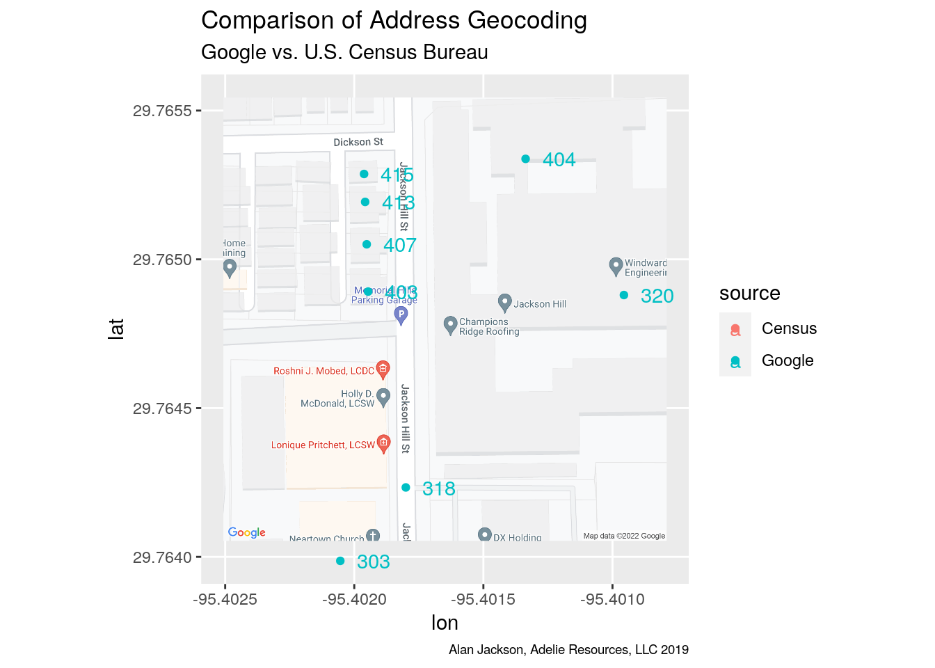
How big is the difference?
Let’s make a table of these differences
#  rearrange the tibble to be organized by address
distance <- function(lat1, lon1, lat2, lon2){
  sqrt((as.numeric(lat1)-as.numeric(lat2))**2 +
       (as.numeric(lon1)-as.numeric(lon2))**2)* 69*5280
  }

loctable <-
  locations %>%
  select(status, match_address, lat, lon, label, source) %>%
  unite(temp, status:lon, sep=":") %>%
  spread(key=source, value=temp ) %>%
  separate(Census, into=c("Census Status",
                          "eraseme",
                          "census_lat",
                          "census_lon"), sep=":") %>%
  separate(Google, into=c("Google Status",
                          "Address",
                          "google_lat",
                          "google_lon"), sep=":") %>%
  mutate(Distance=distance(census_lat, census_lon,
                           google_lat, google_lon)) %>%
  select(-eraseme)


  # display in a nice table

loctable %>%
  select(Address, "Google Status", Distance) %>%
  mutate(Distance=round(Distance,2)) %>%
  gt() %>%
  tab_header(title="Distances between Google and Census locations") %>%
cols_label(Distance="Distance in feet")| Distances between Google and Census locations | ||
|---|---|---|
| Address | Google Status | Distance in feet |
| 303 Jackson Hill St, Houston, TX 77007, USA | ROOFTOP premise | 96.24 |
| 318 Jackson Hill St, Houston, TX 77007, USA | RANGE_INTERPOLATED street_address | 72.51 |
| 320 Jackson Hill St, Houston, TX 77007, USA | ROOFTOP street_address | 340.35 |
| 403 Jackson Hill St, Houston, TX 77007, USA | ROOFTOP street_address | 135.67 |
| 404 Jackson Hill St, Houston, TX 77007, USA | RANGE_INTERPOLATED street_address | 251.10 |
| 407 Jackson Hill St, Houston, TX 77007, USA | ROOFTOP premise | 96.63 |
| 413 Jackson Hill St, Houston, TX 77007, USA | ROOFTOP street_address | 74.28 |
| 415 Jackson Hill St, Houston, TX 77007, USA | ROOFTOP premise | 54.87 |
So differences of 50 - 250 feet!
Part of this is that the Census tries to locate the address at the curb in front of the address (although the cluster of addresses for homes, 403,407, 413, and 415 seems to indicate they are not too good at this), while Google gives a point roughly in the center of the building at that address. I purposely chose an apartment complex to illustrate how bad this can get.
Note the Google Status column. According to Google, ROOFTOP implies “a precise geocode for which we have location information accurate down to street address precision”. RANGE_INTERPOLATED " indicates that the returned result reflects an approximation (usually on a road) interpolated between two precise points“. However, I do not find these especially helpful. 320 is a ROOFTOP location, but because it is a large building, that location is well off the street, so depending on the usage, that could be an issue.
Since the Census locations are based on the Tiger files, they do follow the streets quite well. However, their actual accuracy seems to be quite low.
Other Census Issues
In their documentation, the Census Bureau notes that their data is incomplete - if an address is not in a residential area, they are not interested in it. Queries for much of downtown Houston failed - I assume for this very reason. No one lives there. I am looking at police data, and apparently a lot of crime occurs under freeways. The Census fails to geolocate those addresses.
Another flaw, in my opinion, is how they handle directional prefixes - they are given a very low weighting in their matching algorithm, so when I asked for 1200 N Shepherd, it would return 1200 S Shepherd. An error of several miles. The only way to force it onto the correct part of the street is to supply a zipcode, which I did not have, so I had to expend some effort estimating zipcodes to get it to work.
So why bother with the Census server, why not use Google?
Let’s look a some issues Google has.
Addresses <- c("1520 Tulane St, Houston, TX, 77008",
               "1550 Tulane St, Houston, TX, 77008",
               "1570 Tulane St, Houston, TX, 77008",
               "1600 Tulane St, Houston, TX, 77008",
               "1700 Tulane St, Houston, TX, 77008")

locations <-
tibble( status=character(),
        match_address=character(),
        lat=numeric(),
        lon=numeric(),
        tract= character(),
        block=character())
addys <-
  tibble(Addresses) %>%
  separate(Addresses,",", into=c("street",
                                 "city",
                                 "state",
                                 "zip"))

for (i in 1:nrow(addys)){
 a  <-
  Census_decoder(address=addys[i,]$street,
                 city=addys[i,]$city,
                 state=addys[i,]$state,
                 zip=addys[i,]$zip)
  locations <- bind_rows(a,locations)
}

locations <-
  locations %>%
  mutate(label=str_extract(match_address,"[0-9]*"),
         source="Census")

#   Get locations from Google

register_google(key = googlekey)
for (i in 1:length(Addresses)){
  a <- getfields(geocode(Addresses[i], output="all"))
  a <- a %>%
    mutate(status=paste(LocType, types),
           tract=" ",
           block=" ",
           label=str_extract(match_address,"[0-9]*")) %>%
    select(status, match_address, lat, lon, tract, block, label) %>%
    mutate(source="Google")
  locations <- bind_rows(a,locations)
}

MapCenter <- c(-95.402178, 29.7992)
gmap = get_map(location=MapCenter,
               source="google",
               zoom=zoom,
               maptype="roadmap")

ggmap(gmap, extent='normal', maprange=FALSE, show.legend=FALSE) %+%
  locations + aes(x = lon, y = lat, color=source) +
  geom_point(data=locations) +
  geom_text(aes(x=lon, y=lat, label=label), hjust=-0.5)+
  labs(title="Comparison of Address Geocoding",
       subtitle="Google vs. U.S. Census Bureau",
caption=caption) 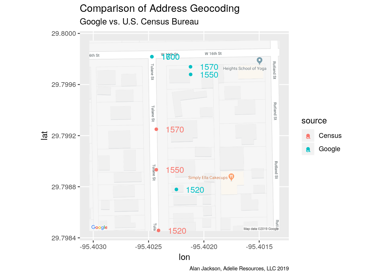
So from the map we can see several things. For example, Google’s tag for 1520 Tulane is spot on (ground truth from streetview). The census data is all shifted rather badly - the north-south blocks in this area have addresses that only go from 0 to 50, that is 1500-1550 on this block, not 1599, which apparently the census data assumes.
So what gives with the Google points at 1570, 1600, and 1700? Those addresses do not exist. The street does not exist for the 1600 and 1700 blocks. But Google returns an answer anyway, that is simply wrong. For 1600 and 1700, the Census query fails. So I would claim that is a good thing. Moreover, Google does not really give you much of a clue about what it has done. The addresses are returned as RANGE_INTERPOLATED, but that can happen with legitimate addresses.
So we have several problems. Google is happy to return adresses that do not exist - where the street does not even exist. The census returns addresses only where the street exists, but assumes addresses go from zero to 99, and so is stymied when they do not.
So let’s summarize:
Google Pro’s
- able to handle dirty data (misspelled streets)
- fairly comprehensive, even for new neighborhoods
- points flagged as “rooftop” are real and exact
Google Con’s
- will happily return nonsense as if it is real
- 2500 query per day limit
- location at building center (for some this could be a Pro)
Census Pro’s
- unlimited daily queries
- will return an error for addresses that do not exist (mostly)
- locations are along curb (for some this could be a Con)
Census Con’s
- input address must be pretty close to correct
- handles directional prefixes poorly
- assumes blocks run from 0-99
- only covers residential addresses (mostly) and not as current
What have I decided to use for my purposes? I have about 100,000 addresses to geocode, so I am trying to do as many as possible with the Census geocoder, and then falling back to the Google geocoder for the remainder. However, I have to do a lot of error checking for both with the output data - for example with Google if I look for 1600 and 1625, does the point move? If not I have a problem.
Other geocoding issues
I have had sporadic server issues with both products. I have had Google fail in such a way that I lost 2000 queries. Because of that I now only call it one query at a time. For a while Google was failing with an erroneous “maximum query reached” message on about 20% of my queries. That was frustrating. And for the Census queries I have set up an automatic retry, because I was seeing enough server failures that it seemed necessary.